The Simple Geometry Behind Any Road

In the last blog post, I explained what sits at the backbone of procedurally generated roads: the data structure, aka the minimum information you need to describe any piece of road infrastructure. The answer to that fundamental question was a set of abstract cross-sections of the road, each storing a snapshot of how the road looks at that specific point (or, should I say, line). I called them simply: profiles.

A good analogy I didn’t have the inspiration to make at the moment was to compare them with Bezier splines. To store a Bezier spline, you don’t need to save the entire curve explicitly, but just anchor points and handle positions. With a bit of math and a few formulas, you can reconstruct the actual path at any time by interpolating between the control points.

The profile-based representation works the same in my system. The profiles are the control information, and the actual geometry defining the road path is the interpolated result of those profiles.

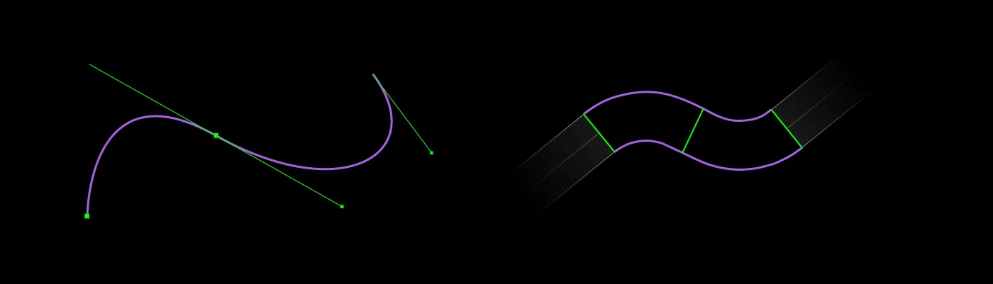
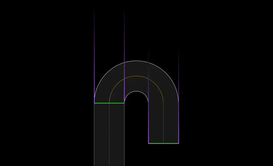
In this blog post, I’ll go over how I am computing the purple part. How to interpolate between these green profiles to generate beautifully smooth, parallel paths?

The Geometry Problem

In my first post, I explained why I embarked on this journey: I found most game devs seemed to be using the wrong tool for the job, rendering roads by expanding a centerline Bezier spline. I knew from the start I wanted to use only lines and circular arcs to build the actual road shape.

With the prerequisites fixed, we reduced our problem to a geometry one:

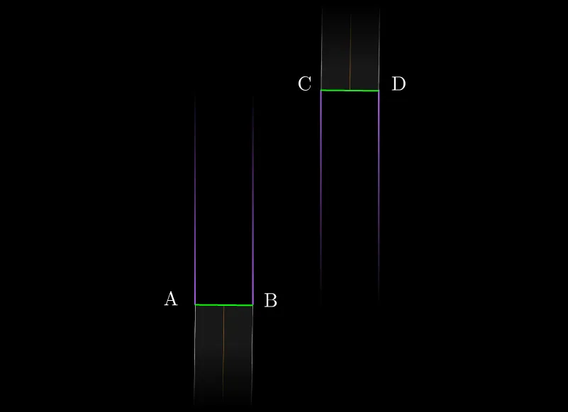
Given two profiles at arbitrary positions and orientations, how do we connect their respective endpoints using smooth parallel arcs?

A simple geometric property of circles instantly gets us one simplification for free. Points equally spaced along a radius trace concentric arcs when rotated around the same center. As long as our profiles are equal in length, we only need to solve the path for one pair of corresponding endpoints. Applying the same construction across the profile naturally results in parallel paths.

The problem is then reduced to:

Given two points $A$ and $B$ with their respective direction vectors $\vec{dA}$ and $\vec{dB}$, find a circular arc that connects $A$ to $B$ and is tangent to $\vec{dA}$ at $A$ and $\vec{dB}$ at $B$.

A Single Arc Won’t Do The Trick

You probably guessed it without jumping into the math. Two arbitrary points, each with a prescribed tangent vector, cannot always be connected by a single circular arc tangent to both vectors. It’s actually more of a special optimal case when they do, meaning the points happen to lie on the same circle.

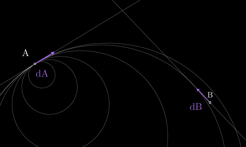
It might look like we’ve backed ourselves into a corner at this point. Constraints we’ve fixed simply can’t be satisfied. But at the same time, in real life, roads do exist, defined only by arcs and lines. The answer is to ease the constraints a bit by letting each arc also have a line extension until it meets the point along the tangent line.

The Geometrical Solution

Here is how the construction unfolds:

1. Take two respective endpoints (let’s denote them $A$ and $B$).
2. From each point, extend a line in the direction the road should continue (perpendicular to the profile). I’ll refer to these as continuation lines.
3. Let’s call the point where these two lines intersect $C$.
4. We now have two segments, $CA$ and $CB$, which differ in length in the general case. Let’s assume $CB$ is longer than $CA$.
5. Starting from $B$ and moving along the continuation line toward $C$, we pick a new point $M$ such that $CM = CA$.
6. From here, draw a line through $M$ that is perpendicular to the second continuation line, and a line through $A$ that is perpendicular to the first.
7. Let these two perpendiculars intersect at a new point, $O$.

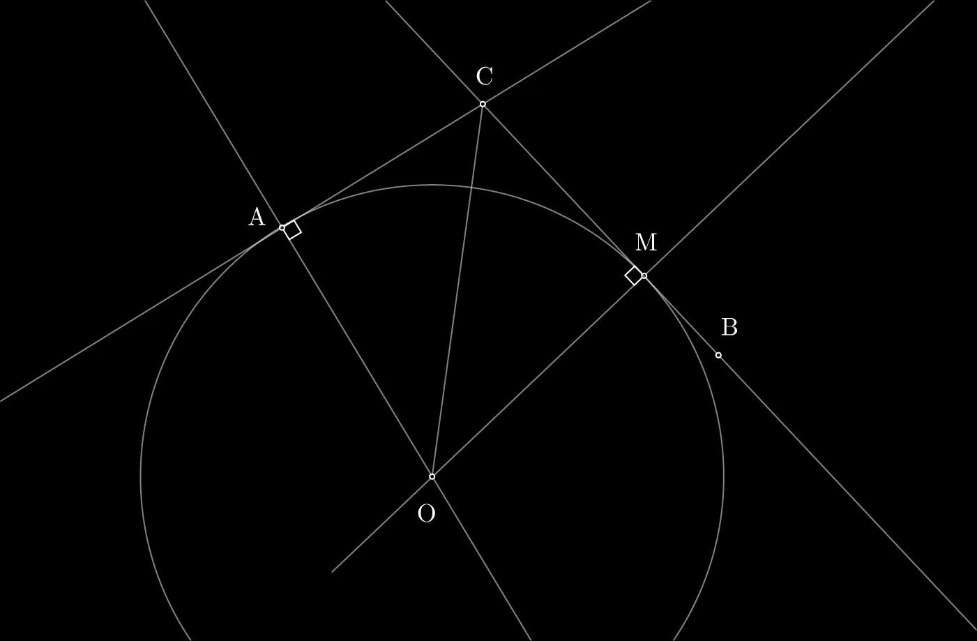
The Tangent–Radius Theorem tells us that a radius is always perpendicular to the tangent at the point of contact. So if $OM$ and $OA$ are radii of the same circle, it means the circle will be tangent to the continuation lines at $M$ and $A$.

The only thing left to do is prove $OM = OA$.

The proof is quite simple. Consider the right-angled triangles $OCM$ and $OCA$ with a common hypotenuse $OC$. Since we chose M so that $CM = CA$, we conclude that the triangles are congruent and that $OM = OA$, proving that $O$ is indeed the center of a circle through M and A.

The final path is therefore an arc from $A$ to $M$ followed by a straight line from $M$ to $B$.

A straight line, then an arc. That’s the whole trick.

Some CAD engineers may read this and chuckle: “That’s just a fillet”. Yes, this thing I’ve just described is nothing new under the sun; it’s called a two-line fillet construction. But with a little twist: one tangential point is always fixed, and the other is solved for. An even more practical way to picture this (especially for people who use tools like Illustrator or Figma) is to think of applying an infinite corner radius to one corner of a shape.

Profiles Interpolation

Now that we have a reliable way to smooth a path between two endpoints with prescribed directions, we can get back to the real problem: connecting a source to a target profile.

In most cases, this is actually very straightforward.

If the two profiles are equal in length and their continuation lines intersect in a reasonable way, then connecting the full profiles is just the same construction applied twice to their corresponding ends. In other words, we solve the same geometry problem on both sides of the road cross-section, and the two edges will run parallel naturally.

So most ordinary road segments boil down to repeating this exact same trick between the start and end profiles. Here is how it unfolds visually:

The Next Problem

Of course, not every valid pair of profiles is angled in such a convenient way that their continuation lines intersect and can form a fillet.

The next block in the road (pun intended) is to solve for other edge cases, which are actually not that edge. The method above just falls apart if those continuation lines do not intersect. Picture the following setup.

This scenario is perfectly valid, as roads don’t just curve, but sometimes they shift.

In other words, a vehicle might be aligned with wheels standing at $AB$ at one moment and needs to smoothly arrive at $CD$. In practice, that means it must first turn one way, then the other, forming an S-like path.

A single arc cannot establish that transition; at least two are required. So a new approach is needed.

The Intermediary Profile

I remembered seeing this exact kind of shift with LEGO train tracks while playing with my daughter.

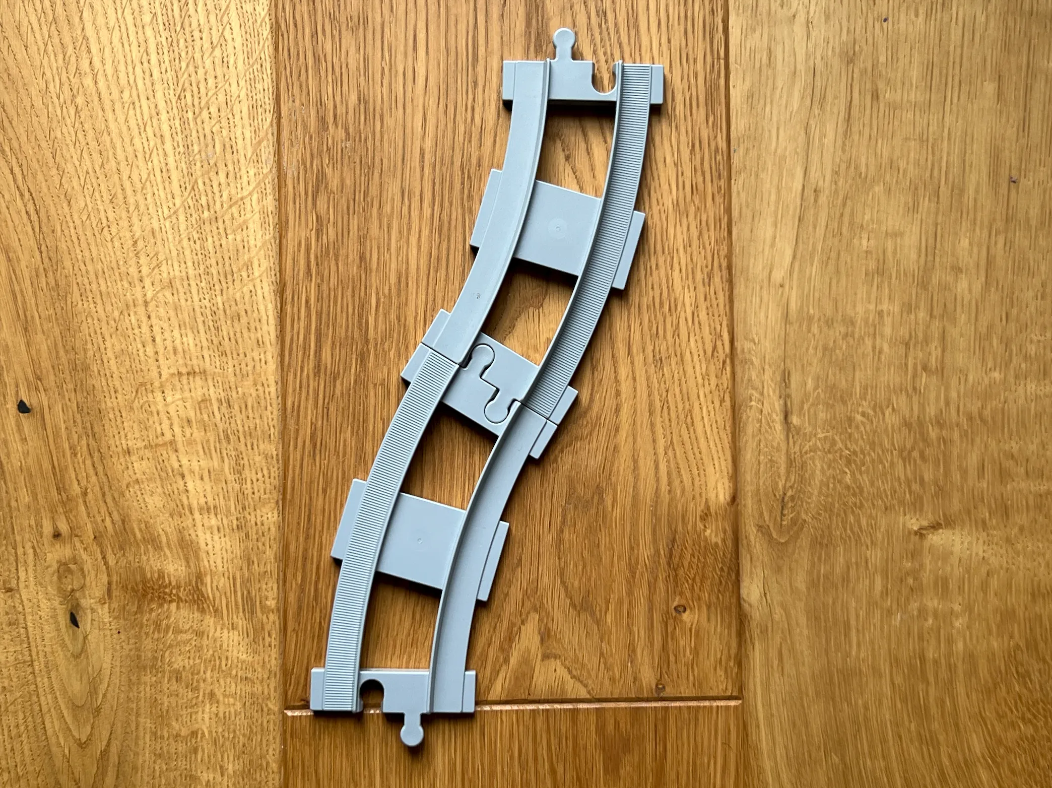
Chaining two arch pieces with opposite turning directions would yield a beautiful S shift transition.

So then I realized: this doesn’t need to be solved in one step: I just need to find a way to connect the same primary building blocks.

The task is to find an intermediary profile somewhere in between that lets me split the problem into two that I already know how to solve using same two ingredients: lines and arcs.

Back to Splines?

Even though I said splines are not a good fit as the primary representation for a road’s shape, they are perfect for one thing: finding a good candidate position and orientation for this intermediary profile.

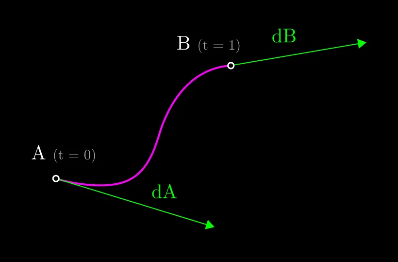
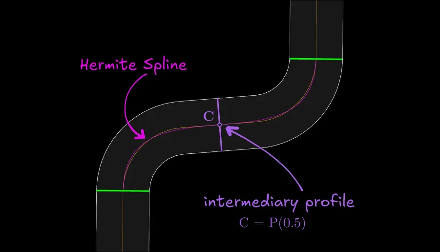
The best match here is the cubic Hermite spline between the center of the source and target profiles.

A cubic Hermite spline takes two points $A, B$ and two tangent vectors $dA, dB$ and smoothly interpolates between them. For $t = 0$, you get the start point. For $t = 1$, you get the endpoint. For any $t$ value in between, you get a smooth path that matches the specified tangent directions at both endpoints.

In theory, the “ideal” place to insert the intermediary profile is at the inflection point, where the curve changes curvature. There is actually a fancy mathematical way to find this exact point by computing the first and second-order derivatives of the spline and solving a 3rd-degree polynomial equation. More details here for those who want to dive deeper.

But I said the math was simple, right? In practice, we really don’t need that precision.

For reasonable magnitudes of $dA$ and $dB$ (roughly between 1.0 and 1.5 times the distance between the center points), simply evaluating the Hermite spline at $t = 0.5$ gives a very good approximation of where that turning transition happens.

Evaluating $P(0.5)$ gives us the profile’s center position. (where $P(t)$ is the parametric form of the Hermite spline)

If, for a Cartesian space function, the first derivative (rise over run) tells you the slope of the plot at a specific x value, then for a 2D parametric curve, the first derivative gives you the velocity vector: how the point moves as t changes. If you think of t as time, this represents both the speed and direction of motion.

In our case, we are only interested in the direction, which is actually the tangent. Simply evaluating $P’(0.5)$ yields the tangent direction at that point along the curve.

From a programming standpoint, $P$ and $P`$ are just some simple formulas that evaluate in O(1).

Special Cases

To this point, we can handle most useful profile-to-profile connections. But there are still a couple of special scenarios worth discussing.

The first one is when the continuation lines are parallel and point in the same direction.

That one actually has a very clean construction: use a half-circle from one side, then a straight segment.

The last annoying family of edge cases is when the continuation lines do not intersect in a way that can be cleanly resolved with a single intermediary profile.

I am fairly sure that, with enough effort, a universal solution can be built for these scenarios as well. I would genuinely love to hear from people who have ideas here.

But sometimes you just need to accept some limitations in your tool and build design constraints that completely prevent the user from ending up in these scenarios.

Constraining by Design

So instead of chasing every impossible arrangement, I chose to build a constraint directly into the road placement tool.

By splitting the plane in half using the infinite line of the source profile, if the user tries to place the next profile in the “behind” half-plane, I force that new profile to match the orientation of the source profile. That reduces the setup to one of the simpler special cases above, which can already connect robustly.

What’s next?

At this point, we have the core building block of the road network: a way to connect two profiles smoothly using only lines and circular arcs.

That gives us the freedom to draw roads in any shape.

The next step is to figure out how to dynamically establish intersections when roads meet and stitch these building blocks together into more intricate networks.

That is what I will go over in the next blog post.

Footnotes

1. In order to understand how to mathematically find this inflection point, we need to think about what the first and second derivatives of a parametric curve tell us about its nature at that point. The first derivative $P'(t)$ will tell us the direction of motion, while the second derivative $P''(t)$ will tell us how that direction changes over time, in other words, how the curve is turning (curvature).

   A good way to picture this is to think of $P'(t)$ as the direction the headlights point in and $P''(t)$ as the direction the steering wheel is turning. The inflection point is the moment when those two align; the curve briefly stops before switching direction.

   To determine whether two vectors are aligned, we can compute their cross product. This is 0 when they either have the same direction or go in opposite directions. So, mathematically, finding the inflection point is equivalent to solving the equation $P'(t)$ ⨯ $P''(t) = 0$

   Back to content ↩